Free Training – Steps How to Work in Work View on Microsoft Excel 2007

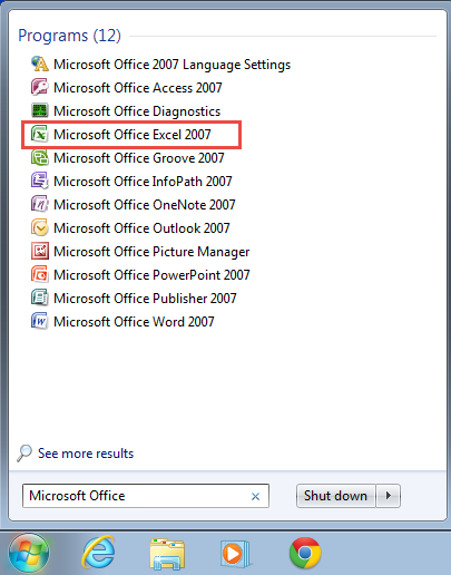
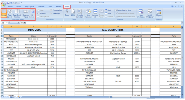
Custom views in MS Excel are used a great deal by professionals who deal with Excel sheet on a daily basis. This feature makes it easy for you to save a set number of display and print settings as “MS Excel Views.” These settings can be readily used by anyone at a later stage. Here is a step-to-step guide on how to work with basic functions and data formulas in MS Excel: Step 1: Go to the “Start” menu and type in Microsoft Excel. Double click on the “Microsoft Office Excel” option to open an MS Excel sheet. (Check the screenshot below)   With MS Excel, you can use one more highly useful option in view – you can also work with workbook views. Step 2: Go to the “View” option and select “Normal.” Here, you can see that the entire sheet is in a “normal” view. 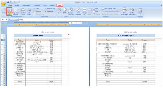(Check the screenshot below)         Step 3: Click on the “View” option. Next, when you click on the “Page Layout” option, you’ll find that you can even change layout of the page. (Check the screenshot below)       You can also use the “Page Break” option in MS Excel. In order to insert a vertical page break: Step 4:Select the row below which you want to insert the page break. To successfully insert a horizontal page break, you will have to select the column that is exactly on the right of the column where you want to insert the page break. 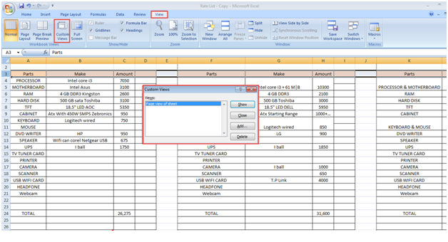(Check the screenshot below) Step 5: You can also see the custom view option here. You can freeze, hide and show all data on the sheet, as you see fit. (Check the screenshot below) Step 6: Here, you will also see that if you click on the “Full Screen” option, the sheet opens in full screen. (Check the screenshot below)       Learning to use custom views in MS Excel is easy and straightforward, right? If you faced any difficulty while working with views in Excel, we’d like to help. Tell us about the problem you are facing in comments and we’d like to provide you with detailed answers.